Rankine earth pressure by finite elements, to six figures
A smooth wall 6 m high retaining a soil with a friction angle of 30 degrees is moved away from and into the ground in the open-source finite element program KATAI 2D, and the force on it is read from the reactions. The at-rest, active and passive forces come out at 162.0000, 108.0000 and 972.0000 kN/m, the Rankine closed forms to every printed digit. Full active pressure needs 4.9 mm of movement and full passive pressure 73.7 mm, fifteen times as much, and with a cohesion of 10 kPa the tension cut-off reproduces the tension-crack formula to 0.06%. The script and the project files are provided.
Rankine’s earth pressure coefficients are the first numbers a geotechnical engineer learns and the last ones anybody checks. This article checks them — not against a textbook, but by building the wall in a finite element program, moving it, and reading the force it carries.
The program is KATAI 2D, which I write and maintain, so read this as a documented verification record rather than an independent review. Everything below was computed with the published release 0.9.0, from one Python script of about a hundred lines that anyone can run. The script also saves each case as a project file that opens in the desktop application.
The short version: the finite element forces equal the closed forms to the last printed digit, which is what should happen and is worth seeing happen. The more useful results are the two that a coefficient does not tell you: how far the wall has to move, and what cohesion does when the soil cannot carry tension.
1. The problemPermalink to “1. The problem”
A vertical wall of height retains soil with a horizontal surface. The wall is smooth — it transmits no shear — and so is the base the soil rests on. The far end of the block is a roller. Under those conditions a horizontal movement of the wall strains the whole block uniformly, the principal stresses stay vertical and horizontal, and every point reaches failure in the same state Rankine assumed.
That makes the closed forms exact for this boundary value problem, not approximations of it:
and before the wall moves at all the soil is at rest, with Jaky’s coefficient:
1.1 InputsPermalink to “1.1 Inputs”
| Symbol | Value | Unit | Meaning |
|---|---|---|---|
| 6 | m | wall height | |
| 12 | m | length of the retained block | |
| 18 | kN/m³ | unit weight | |
| 30 | ° | friction angle (associated flow, ) | |
| 0, then 10 | kPa | cohesion | |
| 40 000 | kPa | Young’s modulus | |
| 0.3 | – | Poisson’s ratio |
With the coefficients are round numbers, which is why the example uses it: , , . The reference quantity is 324 kN/m, so the three closed-form forces for the cohesionless case are 162, 108 and 972 kN/m.
2. The modelPermalink to “2. The model”
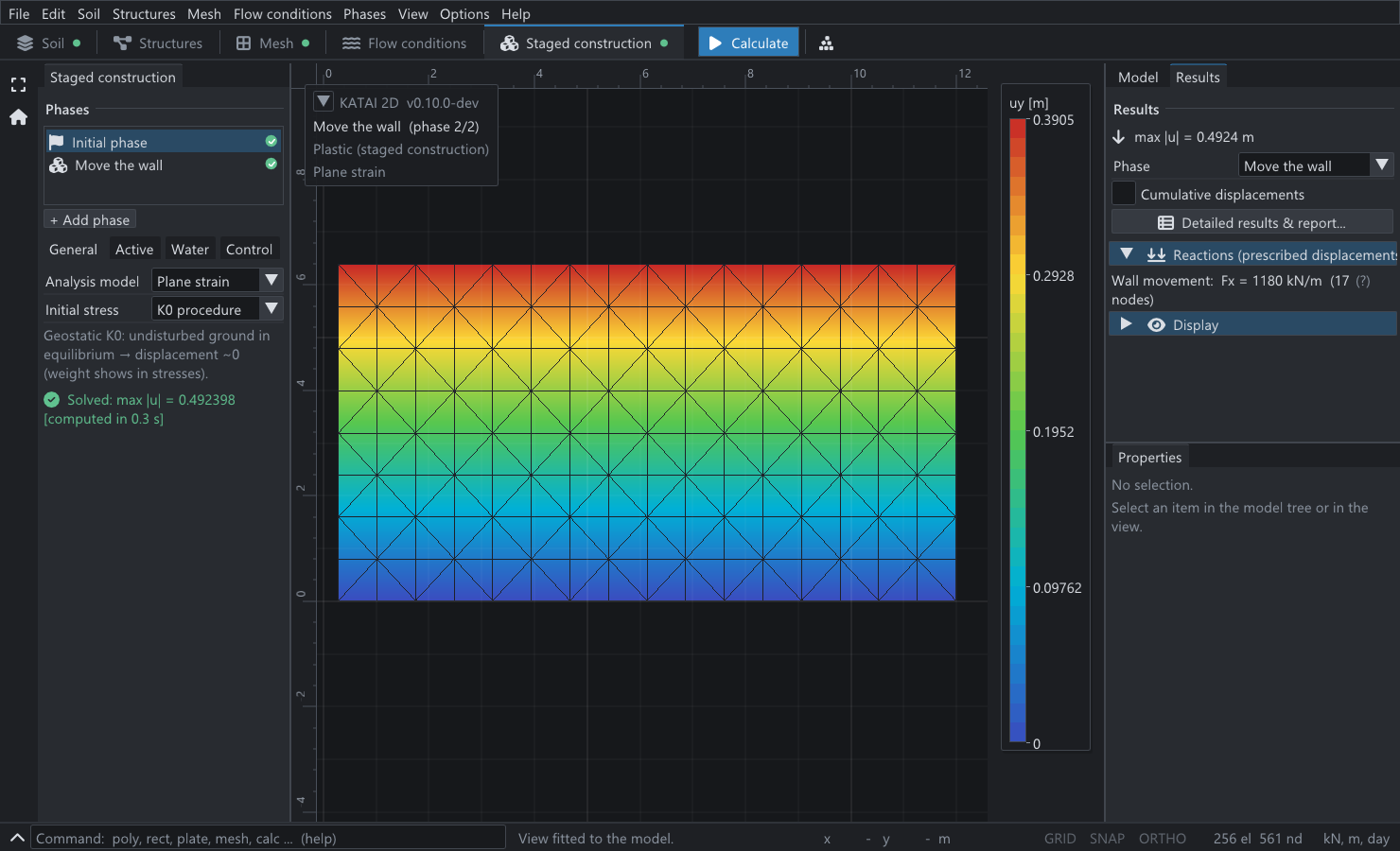
The whole model is one rectangle and one prescribed displacement:
import katai

prj = katai.Project("Rankine wall", mesh_size=1.0, auto_refine=False)
soil = prj.materials.mohr_coulomb("Soil", E=4.0e4, nu=0.3, c=0.0, phi=30.0, psi=30.0,
                                  gamma=18.0)

# Edges in order: base, far side, surface, wall.
# "vertical" holds u_y only (a smooth base); "horizontal" holds u_x only (a roller).
prj.geometry.polygon([(0, 0), (12, 0), (12, 6), (0, 6)], material=soil,
                     fix=["vertical", "horizontal", "free", "horizontal"])
wall = prj.displacements.line((0, 0), (0, 6), ux=-0.005, name="Wall movement")

prj.initial(procedure="k0", exclude=[wall])          # at rest
prj.phases.plastic("Move the wall", activate=[wall])

at_rest, moved = prj.run().results()
Two details carry the physics. The wall is not a structural element: it is the left edge of the soil, held horizontally in the initial phase and then given a prescribed horizontal displacement — negative to move away from the soil, positive to move into it. And the vertical displacement on that edge is left free, which is what “smooth” means.
The force on the wall is the sum of the horizontal reactions at the nodes on :
import numpy as np

on_wall = np.abs(np.asarray(moved.node_x)) < 1e-9
P = abs(np.asarray(moved.reaction).reshape(-1, 2)[on_wall, 0].sum())
The initial phase uses the procedure, which sets the horizontal effective stress to times the vertical one and generates no displacement. If no is given the program takes Jaky’s value from the friction angle, so the at-rest force is a check on the initial state and costs nothing extra.
3. Sand: three states, three forcesPermalink to “3. Sand: three states, three forces”
For , the wall is moved 5 mm away from the soil in one run and 300 mm into it in another:
| State | KATAI 2D 0.9.0 | Closed form | Difference |
|---|---|---|---|
| At rest, | 162.0000 kN/m | 162.0000 kN/m | +0.0000% |
| Active, | 108.0000 kN/m | 108.0000 kN/m | +0.0000% |
| Passive, | 972.0000 kN/m | 972.0000 kN/m | −0.0000% |
The agreement is not luck and it is not tuning. The exact stress field is linear in depth, and a six-node triangle represents a linear stress field exactly; the element size therefore does not matter here. What the table checks is everything else: the initial stress procedure, the Mohr–Coulomb return to the yield surface, the flow rule and the recovery of reactions from the stresses. Any of them being slightly wrong would show in the fourth digit.
4. How far does the wall have to move?Permalink to “4. How far does the wall have to move?”
A coefficient says what the pressure is at failure. It does not say how much movement gets you there — and that is what decides whether a design may count on passive resistance at all.
The same script moves the wall by a series of amounts and records the force each time:
| Wall movement | Force | ||
|---|---|---|---|
| −5.0 mm (away) | −0.083% | 108.000 kN/m | 0.3333 |
| −2.0 mm | −0.033% | 126.986 kN/m | 0.3919 |
| −1.0 mm | −0.017% | 142.274 kN/m | 0.4391 |
| −0.5 mm | −0.008% | 151.548 kN/m | 0.4677 |
| 0 (at rest) | 0 | 162.000 kN/m | 0.5000 |
| +5.0 mm (into the soil) | +0.083% | 267.940 kN/m | 0.8270 |
| +20.0 mm | +0.333% | 542.265 kN/m | 1.6737 |
| +50.0 mm | +0.833% | 887.945 kN/m | 2.7406 |
| +100.0 mm | +1.667% | 972.000 kN/m | 3.0000 |
| +300.0 mm | +5.000% | 972.000 kN/m | 3.0000 |
The active state is fully developed after 5 mm. The passive state is not there at 50 mm and is there at 100 mm. Both thresholds can be derived, and the derivation explains the asymmetry.
4.1 The thresholds in closed formPermalink to “4.1 The thresholds in closed form”
While the soil is elastic, a uniform horizontal strain at constant vertical stress changes the horizontal stress by , where is the plane-strain modulus — here 43 956 kPa. Yield is reached at depth when that change equals the gap between the at-rest stress and the failure stress, . The gap grows with depth, so the surface yields first and the base last; the whole wall is at failure when the base is:
The ratio is . Passive resistance needs fifteen times the movement of active pressure in this soil, for no reason other than that the passive failure stress is fifteen times further from the at-rest stress.
Between zero and the threshold, the soil above the depth has yielded and the soil below it has not, and the force is the sum of the two parts:
with the plus sign for movement into the soil. Evaluated at the intermediate movements of the table it gives 126.989, 142.258 and 151.570 kN/m on the active side and 268.163, 541.927 and 888.190 kN/m on the passive side. The finite element values are within 0.09% of every one of them, and here the mesh does matter slightly: the boundary between yielded and elastic soil falls inside an element.
The practical reading is the familiar one, now with a number on it. A retaining wall reaches active pressure with a movement nobody would notice — less than a tenth of a percent of its height in this example — while passive resistance in front of it needs more than one percent. A design that adds full active load to full passive resistance is adding two things that do not exist at the same displacement.
5. Cohesion, and the tension the soil does not havePermalink to “5. Cohesion, and the tension the soil does not have”
Give the same soil a cohesion of 10 kPa. The passive side is unremarkable:
and the finite element force is 1179.8461 kN/m.
The active side is where the formula and the soil part company. The Rankine expression gives 38.7180 kN/m, but it gets there by letting the upper part of the soil pull on the wall: the active stress is negative down to a depth
Soil does not pull on walls. The textbook correction is to ignore the tension zone — a tension crack — and take the pressure of the soil below it:
which is 28.7% more load than the uncorrected formula.
A finite element model makes the same choice through its tension cut-off: a limit on how tensile a principal stress may become, zero by default in KATAI 2D as in most geotechnical programs. Run both ways:
| Active case, = 10 kPa | KATAI 2D 0.9.0 | Closed form | Difference |
|---|---|---|---|
| Tension allowed (cut-off off) | 38.7180 kN/m | 38.7180 kN/m | +0.0001% |
| No tension (cut-off on, the default) | 49.8587 kN/m | 49.8291 kN/m | +0.0594% |
With the cut-off switched off the model reproduces the formula that allows tension; with it on, the formula with the crack. Nobody told the program where the crack is. The 0.06% that remains in the second row is discretisation — the depth 1.9245 m does not coincide with a row of nodes on a 1 m mesh.
This is the part worth remembering when reading any finite element result for a cohesive soil: the default answer already contains the tension crack. Comparing it with the uncorrected Rankine or Coulomb formula will show a difference of tens of percent that is not an error in either.
6. What happens if you push it too farPermalink to “6. What happens if you push it too far”
One run in the series was refused. Moving the wall 20 mm away from the cohesionless soil — four times the movement that already produced the full active state — the program stopped and reported that the tangent stiffness had gone singular along a mechanism.
That is the correct answer. A block of cohesionless, perfectly plastic soil that is at failure at every point has no stiffness left with which to define a further increment of displacement, and a prescribed movement into that state has no unique solution. With cohesion the same run converges, because the cut-off zone near the surface leaves the problem well posed. The force at 5 mm is the active force; asking for 20 mm adds nothing to it.
I mention it because a refusal is information. A program that had returned a number for that run would have been returning the number its damping, its tolerance or its last converged step happened to produce.
7. What this does and does not establishPermalink to “7. What this does and does not establish”
- It establishes that the initial stress procedure, the Mohr–Coulomb integration with associated flow, the tension cut-off and the reaction recovery are mutually consistent to round-off on a problem with an exact solution, and that the development of plastic zones under increasing movement follows the closed-form transition to within 0.09%.
- It does not establish anything about rough walls. Wall friction rotates the principal stresses, the stress field is no longer homogeneous, and the reference becomes a limit analysis solution rather than Rankine’s. That is a different benchmark.
- The movements are those of this soil and this geometry. They scale with . A stiffer soil or a shorter block reaches both states sooner; the ratio of fifteen between them depends only on the friction angle.
- The elastic–perfectly plastic model has one stiffness. Real passive resistance mobilises along a curve, and real unloading is stiffer than first loading. The thresholds here are a lower bound on how gradual the transition is, not a prediction for a particular wall.
8. Reproducing thisPermalink to “8. Reproducing this”
| What | Where |
|---|---|
| Script | rankine_earth_pressure.py |
| Project files written by it | rankine-sand-active.k2d, rankine-sand-passive.k2d, rankine-clayey-active.k2d, rankine-clayey-passive.k2d |
| Program | KATAI 2D 0.9.0, the published wheel, in a clean virtual environment |
| Run time | under a minute for all fourteen analyses |
> pip install katai2d-0.9.0-cp312-abi3-win_amd64.whl
> python rankine_earth_pressure.py
Ka = 0.333333   Kp = 3.000000   K0 = 0.500000

1. Sand (c = 0)
   at rest   P0 =   162.0000 kN/m   closed form   162.0000   +0.0000 %
   active    Pa =   108.0000 kN/m   closed form   108.0000   +0.0000 %
   passive   Pp =   972.0000 kN/m   closed form   972.0000   -0.0000 %
...
3. Soil with cohesion (c = 10 kPa); tension crack depth zc = 1.9245 m
   passive                 Pp =  1179.8461   closed form  1179.8461   -0.0000 %
   active, tension allowed Pa =    38.7180   closed form    38.7180   +0.0001 %
   active, no tension      Pa =    49.8587   closed form    49.8291   +0.0594 %
The project files can be solved without Python as well: katai solve rankine-sand-passive.k2d. Every figure quoted on this page is recomputed from its stated
inputs by a script that runs on each build of this site, the same arrangement as the
rigid footing benchmark.
ReferencesPermalink to “References”
- Rankine, W. J. M. (1857). On the stability of loose earth. Philosophical Transactions of the Royal Society of London 147, 9–27. — the active and passive states.
- Jaky, J. (1944). The coefficient of earth pressure at rest. Journal of the Society of Hungarian Architects and Engineers 78(22), 355–358. — .
- Terzaghi, K. (1943). Theoretical Soil Mechanics. New York: Wiley. — the tension crack and the earth pressure of cohesive soils.
- KATAI 2D 0.9.0. github.com/fkkarakurt/katai2d, Apache-2.0. doi.org/10.5281/zenodo.20692282.