Reproducing a PLAXIS 2D benchmark to within 0.03%
The PLAXIS 2D Validation Manual publishes a smooth rigid strip footing on an elastic layer with an analytical reference force of 15.15 kN/m and a computed force of 15.24 kN/m. Solved from a checked-in input file, KATAI 2D returns 15.32 kN/m on that file's own mesh and 15.24 kN/m once the discretisation error is resolved by nested refinement — 0.03% from the published value, inside a numerical uncertainty band of 0.21% estimated by the Grid Convergence Index. This article states every input, the analytical formula, the refinement study and the limits of the comparison.
Two finite element programs solving the same boundary value problem should agree, and the useful question is never whether they agree exactly — they cannot — but by how much, and whether that difference is explained. This article works one benchmark through in full: the smooth rigid strip footing on an elastic layer published in the PLAXIS 2D Validation Manual, solved in KATAI 2D, with the analytical solution, every input, the mesh-convergence study and the residual differences all stated. KATAI 2D is software I write and maintain, so read this as a documented verification record rather than an independent review.
The short version: on the input file’s own mesh the computed footing force is 0.53% above the published PLAXIS value; with the discretisation error resolved by systematic refinement it is 0.03% above it, and the remaining difference is smaller than the precision of the analytical coefficient the benchmark itself is built on.
1. The benchmarkPermalink to “1. The benchmark”
A rigid, smooth strip footing of half-width is pressed a settlement into a homogeneous, isotropic, weightless elastic layer. The quantity of interest is the force per metre run the footing carries at that settlement.
Because the footing is rigid, the settlement is uniform beneath it and the contact pressure is not; because it is smooth, no shear is transmitted at the contact. The classical solution for the resulting force on an elastic layer of finite depth is written with a dimensionless coefficient that depends on the layer geometry and Poisson’s ratio, tabulated by Giroud:
with the Young’s modulus of the layer. The PLAXIS 2D Validation Manual publishes this case in its Section 2.1 with and the inputs in the table below, giving an analytical reference of 15.15 kN/m, against which it reports its own computed value of 15.24 kN/m — a difference of 0.6%.
1.1 Inputs, and where each one comes fromPermalink to “1.1 Inputs, and where each one comes from”
Every number below is either published in that section of the manual or derived from one that is, by the arithmetic shown.
| Symbol | Value | Unit | Where it comes from |
|---|---|---|---|
| 500 | kPa | Published input (shear modulus of the layer) | |
| 1/3 | — | Published input (Poisson’s ratio) | |
| 1333.33 | kPa | Derived: | |
| 1 | m | Published input (footing half-width; the footing is 2 m wide) | |
| 10 | mm | Published input (imposed settlement) | |
| 0.88 | — | Published coefficient for this layer geometry (Giroud’s tables) | |
| Layer depth | 4 | m | Published input |
| Model width | 7 | m | Published input (half model; the left edge is the symmetry axis) |
| Unit weight | 0 | kN/m³ | Published input — the layer is weightless, so the footing force is the only load |
Substituting:
The precision of that reference matters, and is easy to miss. The coefficient is
published as 0.88 — two decimals. Everything the coefficient can mean, , maps to a reference force between 15.07 and 15.24 kN/m. The analytical
value of this benchmark is therefore known to about before any finite element
program is opened. Keep that interval in mind; both programs land inside it.
2. The KATAI 2D modelPermalink to “2. The KATAI 2D model”
The problem is expressed as a .k2d input file, checked into the repository as
tests/corpus/kv-fnd-012-giroud-rigid-footing.k2d, so what is described here and what is
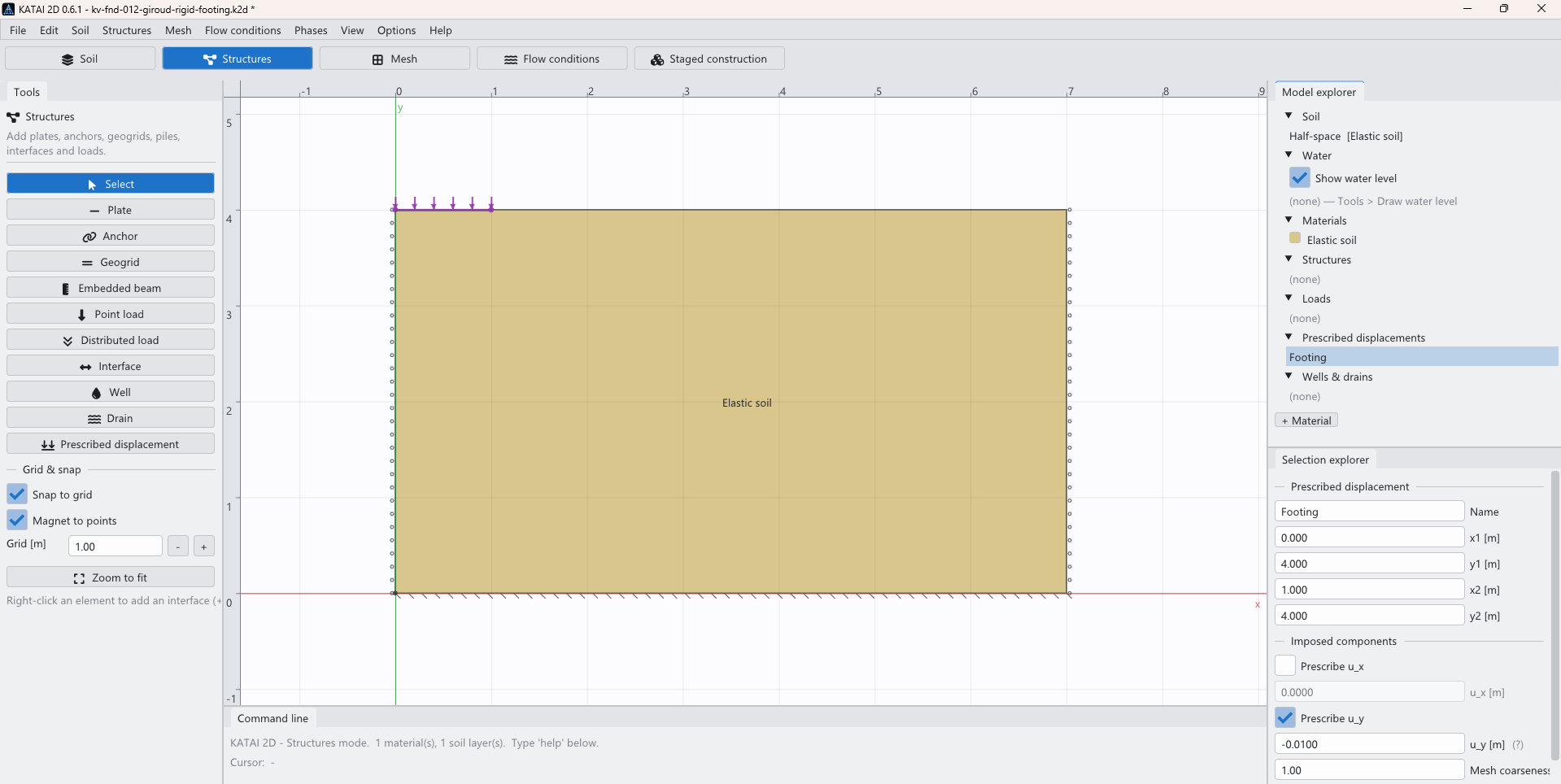
solved are the same bytes. The rigid smooth footing is imposed as a line prescribed
displacement: the vertical component is set to mm on the footing line and
the horizontal component is left free, which is exactly what “rigid” and “smooth” mean.
The force is then read back as the reaction — the internal force of the constrained
degrees of freedom, recovered from the committed stresses as ,
not as an applied load.
| Model item | As built |
|---|---|
| Domain | 7 m × 4 m, half model with the symmetry axis at |
| Element | 15-node triangle (quartic displacement field) |
| Constitutive model | Linear elastic, kPa, , |
| Footing | Prescribed displacement line, m at m, mm, free |
| Boundaries | Base fixed, sides on rollers, surface free |
| Phases | Initial (weightless gravity, no displacement) → indentation |
| Reported quantity | $F = 2\left |
Because the layer is weightless, the initial phase must produce exactly zero displacement, and the automated suite asserts that: a non-zero initial state would mean the reference configuration is not the one the analytical solution assumes. It also asserts that a footing node carries exactly the imposed 10 mm, which is what makes the reaction the force of this problem rather than of a slightly softer one.
3. Running itPermalink to “3. Running it”
The input file is solved by the command-line program, with no graphical step involved:
$ katai info
KATAI 2D 0.6.1 (2026-08-07)
  .k2d project file version: 12
  .res results file version: 5
  linear solver backend: pardiso

$ katai validate tests/corpus/kv-fnd-012-giroud-rigid-footing.k2d
OK: tests/corpus/kv-fnd-012-giroud-rigid-footing.k2d satisfies the input contract (0 warning(s))

$ katai solve tests/corpus/kv-fnd-012-giroud-rigid-footing.k2d
phase 1/2: Initial phase
phase 2/2: Indent
phase 1/2: ok  max|u| = 0.000000e+00 m
phase 2/2: ok  max|u| = 1.008461e-02 m
solved 2 phase(s) in 0.51 s
The footing force is summed from the reaction field:
import katai

pr, notes = katai.load_project("tests/corpus/kv-fnd-012-giroud-rigid-footing.k2d")
r = katai.run(pr).results()[-1]
Ry = sum(r.reaction[2*n + 1] for n in range(len(r.node_x))
         if r.node_y[n] > 4 - 1e-6 and r.node_x[n] <= 1 + 1e-6)
print(f"F = {2*abs(Ry):.2f} kN/m")   # 15.32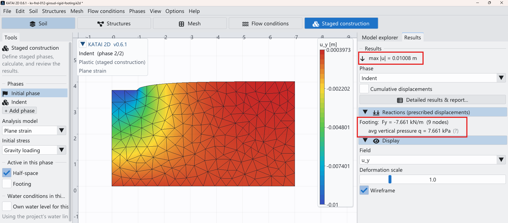
4. How much of the difference is the mesh?Permalink to “4. How much of the difference is the mesh?”
A single number on a single mesh cannot separate the model’s error from the mesh’s. The standard instrument for that is a systematically refined mesh triplet and the Grid Convergence Index, and it requires refinement that is nested: an unstructured mesher that rebuilds the mesh from scratch at each density produces meshes whose differences are not a clean function of element size, and the observed order then comes out at values no element can deliver. Here each mesh is produced from the previous one by uniform (“red”) refinement — every triangle into four similar children — so the refinement ratio is exactly 2 and every angle is preserved.
| Mesh | Elements | Nodes | [m] | [kN/m] | vs analytic | vs PLAXIS 2D |
|---|---|---|---|---|---|---|
| The file’s own | 349 | 2 895 | 0.28325 | 15.32129 | +1.13% | +0.53% |
| Refined once | 1 396 | 11 373 | 0.14162 | 15.26995 | +0.79% | +0.20% |
| Refined twice | 5 584 | 45 081 | 0.07081 | 15.24430 | +0.62% | +0.03% |
with the representative cell size . The estimator returns:
| Quantity | Value |
|---|---|
| Refinement ratios , | 2.0000, 2.0000 |
| Observed order of convergence | 1.0008 |
| Behaviour | monotonic convergence |
| Richardson extrapolation | 15.21867 kN/m |
| Asymptotic ratio | 0.9983 |
| Numerical uncertainty of the fine mesh (GCI, ) | ±0.21% |
Three things in that table are worth reading slowly.
The convergence is monotone and in the asymptotic range. The asymptotic ratio is 0.9983, i.e. within 0.2% of unity, which is the condition under which the observed order may be trusted and the extrapolation quoted at all. Where that condition fails — and on unstructured meshes it often does — the honest response is to fall back on an assumed order with a safety factor of 3 and to refuse to quote an extrapolated value. It does not fail here.
The observed order is 1, not 3. A quartic element on a smooth problem does much better: the same estimator, on the same program, returned for a vertical stress and for a settlement under a distributed strip load. The difference is the punch. A rigid footing carries a stress singularity at its edge, and the integrated reaction inherits it: first-order convergence is what the singularity leaves. This is also the explanation for the sign of the error — every mesh reads high, and refining brings the force down.
The converged value coincides with the published one. At 15.24430 kN/m against a published 15.24 kN/m, the two programs agree to 0.03% — three significant figures — with the residual an order of magnitude inside the ±0.21% numerical uncertainty of the KATAI value. The comparison cannot resolve a difference that small, and it should not be claimed to.
5. The comparison, stated fullyPermalink to “5. The comparison, stated fully”
| [kN/m] | vs analytic 15.15 | vs PLAXIS 2D 15.24 | |
|---|---|---|---|
| Analytical (Giroud coefficient ) | 15.15 | — | −0.6% |
| PLAXIS 2D (published, same section) | 15.24 | +0.6% | — |
| KATAI 2D, the file’s own mesh | 15.32 | +1.1% | +0.5% |
| KATAI 2D, mesh-converged, ±0.21% | 15.24 | +0.6% | +0.03% |
| KATAI 2D, Richardson limit | 15.22 | +0.4% | −0.1% |
And the point made in §1.1 closes the argument: with — the lower end of
what a coefficient printed as 0.88 can mean — the analytical force is 15.24 kN/m, which
is the converged KATAI value to 0.04% and the published PLAXIS value to 0.01%. Both
programs sit inside the precision of the tabulated coefficient the benchmark is defined
by. Beyond that point the benchmark cannot discriminate between them, and any claim that
one is closer to the truth than the other is a claim about rounding.
6. What this does and does not establishPermalink to “6. What this does and does not establish”
It establishes that, on this problem, KATAI 2D solves the elasticity boundary value problem the benchmark poses and lands where an independent, established implementation lands, with the difference quantified and bounded rather than asserted.
It does not establish agreement in general. Specifically:
- One problem, one class of behaviour. This is linear elasticity with a prescribed displacement. Nothing here speaks for plasticity, consolidation, dynamics or staged construction, each of which is verified separately in the KATAI 2D verification suite against its own reference.
- The meshes are not the same meshes. The problem statement is identical; the discretisations are not, and cannot be — which is precisely why the refinement study is here.
- PLAXIS 2D was not re-run. Its value is quoted from its own published validation section. Nothing in this article is a measurement of PLAXIS.
- Agreement is not correctness. Two programs can be wrong together. The analytical solution is the anchor, and it carries the coefficient precision discussed above.
7. Reproducing thisPermalink to “7. Reproducing this”
Everything above is reproducible from the repository:
| What | Where |
|---|---|
| Input file | tests/corpus/kv-fnd-012-giroud-rigid-footing.k2d |
| Automated case | KV-FND-012 in the verification matrix, re-asserted on every build |
| Refinement study | tests/study_giroud_convergence.cpp (cmake --build . --target study_giroud_convergence) |
| Convergence estimator | Grid Convergence Index after Roache (1994) and Celik et al. (2008), in the ASME V&V 20 sense |
| Program version | KATAI 2D 0.6.1, PARDISO backend |
The estimator itself is verified against manufactured triplets whose exact answer is known before it is used on a real one — an error estimator that has not been tested is another unverified number. Every figure quoted on this page is likewise recomputed from its stated inputs by a script that runs on each build of this site, the same arrangement as the Mohr circle construction: a claim that numbers are checked is either enforced or it is decoration.
ReferencesPermalink to “References”
- Giroud, J.-P. (1972). Tables pour le calcul des fondations, Vol. 1. Paris: Dunod. — the tabulated coefficient .
- PLAXIS 2D Validation Manual, Version 8, Section 2.1, “Smooth rigid strip footing on elastic soil”. Bentley Systems / Seequent. — the benchmark statement, the analytical reference force of 15.15 kN/m and the computed value of 15.24 kN/m quoted here.
- Roache, P. J. (1994). Perspective: A method for uniform reporting of grid refinement studies. Journal of Fluids Engineering 116(3), 405–413.
- Celik, I. B., Ghia, U., Roache, P. J., Freitas, C. J., Coleman, H., Raad, P. E. (2008). Procedure for estimation and reporting of uncertainty due to discretization in CFD applications. Journal of Fluids Engineering 130(7), 078001.
- ASME V&V 10-2006, Guide for Verification and Validation in Computational Solid Mechanics; ASME V&V 20-2009 (R2016) for the numerical-uncertainty framework.