Two clay layers, two failure mechanisms, one FE model
Example 4 of Griffiths and Lane (1999) is an undrained clay slope standing on a foundation layer whose strength is varied. Rerun in the open-source finite element program KATAI 2D, the factor of safety rises from 0.8028 at a strength ratio of 0.5 to 1.4286 at a ratio of 1 and then stops at 2.0063 for every ratio from 1.75 upwards. The two classical values are Taylor's 1.47 and 2.10, and the change from a deep-seated to a toe mechanism falls at a ratio of 1.48 against the paper's 1.5. No slip surface is assumed at any point; the script and project files are provided.
A slope stability program based on limit equilibrium has to be told what kind of failure to look for: a circle through the toe, a circle tangent to a firm base, a wedge along a weak seam. On a homogeneous slope the choice is easy. The interesting cases are the ones where two different mechanisms have nearly the same factor of safety, because there the answer depends on whether the analyst thought of both.
Griffiths and Lane’s 1999 paper, which did much to make finite element strength reduction a routine tool, contains an example built to show exactly that. This article reruns it in KATAI 2D — software I write and maintain, so read it as a documented verification record rather than an independent review — using the published release 0.9.0 and a script of about fifty lines.
1. The problemPermalink to “1. The problem”
A slope of height and inclination 2:1 (26.57°) is cut in clay with undrained shear strength . It stands on a foundation layer of the same thickness and a different strength , which in turn rests on a firm base. The analysis is undrained and in total stress: , and the strength of the slope clay is fixed by
The only thing that changes from one analysis to the next is the ratio .
Two classical results bracket the behaviour, both from Taylor’s (1937) stability charts as quoted in the paper:
| Case | Mechanism | Factor of safety |
|---|---|---|
| deep-seated circle tangent to the firm base | 1.47 | |
| circle through the toe, confined to the slope | 2.10 |
Between them something has to give. A weak foundation invites the failure to dive through it; a strong one forces it to stay in the slope. The paper reports the change at a strength ratio of about 1.5, and observes that a limit equilibrium search restricted to one family of circles would miss it.
1.1 InputsPermalink to “1.1 Inputs”
| Symbol | Value | Unit | Where it comes from |
|---|---|---|---|
| 10 | m | chosen; the problem is dimensionless in | |
| 20 | kN/m³ | chosen | |
| 50 | kPa | , the paper’s value | |
| 25 … 150 | kPa | ratios 0.5 to 3 | |
| 0 | ° | undrained, total stress | |
| Geometry | crest , face , toe | – | the paper’s Figure 9 |
| , | 100 000 kPa, 0.3 | – | chosen; a factor of safety does not depend on them |
2. The modelPermalink to “2. The model”
import katai

H, GAMMA = 10.0, 20.0
CU1 = 0.25 * GAMMA * H

def slope(ratio, mesh_size=1.5):
    prj = katai.Project(f"Griffiths & Lane (1999) Example 4, cu2/cu1 = {ratio:g}",
                        mesh_size=mesh_size, auto_refine=False)
    upper = prj.materials.mohr_coulomb("Slope clay", E=1.0e5, nu=0.3,
                                       c=CU1, phi=0.0, gamma=GAMMA)
    lower = prj.materials.mohr_coulomb("Foundation clay", E=1.0e5, nu=0.3,
                                       c=ratio * CU1, phi=0.0, gamma=GAMMA)

    prj.geometry.polygon([(0, 0), (6 * H, 0), (6 * H, H), (0, H)],
                         material=lower, name="Foundation",
                         fix=["full", "horizontal", "free", "horizontal"])
    prj.geometry.polygon([(0, H), (4 * H, H), (2 * H, 2 * H), (0, 2 * H)],
                         material=upper, name="Slope",
                         fix=["free", "free", "free", "horizontal"])

    prj.initial(procedure="safety")     # strength reduction on the gravity state
    return prj

for ratio in (0.5, 0.75, 1.0, 1.25, 1.5, 1.75, 2.0, 3.0):
    prj = slope(ratio)
    prj.save(f"clay-slope-cu-ratio-{ratio:g}.k2d")
    print(ratio, prj.run().results()[-1].fos)
Two polygons, two materials, one loop. The undrained clay is a Mohr–Coulomb material with and its cohesion set to the undrained strength. The base is fixed, the two vertical sides are on rollers, and the mesh is 2576 nodes of six-node triangles at a target element size of 1.5 m.
Nothing in the model says where failure will occur. The strength reduction divides both cohesions by the same trial factor and raises it until equilibrium can no longer be found; the displacement field at that point is the mechanism.
3. ResultsPermalink to “3. Results”
| Factor of safety, KATAI 2D 0.9.0 | Change from the previous row | |
|---|---|---|
| 0.50 | 0.8028 | |
| 0.75 | 1.1214 | +0.3186 |
| 1.00 | 1.4286 | +0.3072 |
| 1.25 | 1.7276 | +0.2990 |
| 1.50 | 2.0031 | +0.2755 |
| 1.75 | 2.0063 | +0.0032 |
| 2.00 | 2.0063 | 0.0000 |
| 3.00 | 2.0063 | 0.0000 |
The table has two regimes and a sharp corner between them.
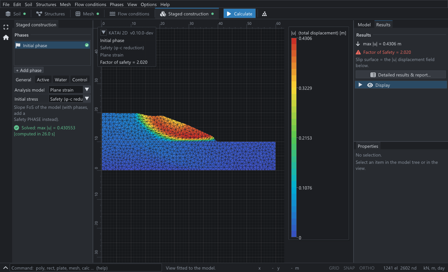
Up to a ratio of 1.5 the factor of safety climbs by about 0.3 for every quarter added to the ratio: the foundation is taking part in the failure, so strengthening it helps. From 1.75 onwards the factor does not move in the fourth decimal place. The foundation has dropped out of the problem. A slope that fails through its toe does not know how strong the ground beneath it is.
3.1 Against the classical valuesPermalink to “3.1 Against the classical values”
| Case | Taylor (1937) | KATAI 2D 0.9.0 | Difference |
|---|---|---|---|
| , base failure | 1.47 | 1.4286 | −2.8% |
| , toe failure | 2.10 | 2.0063 | −4.5% |
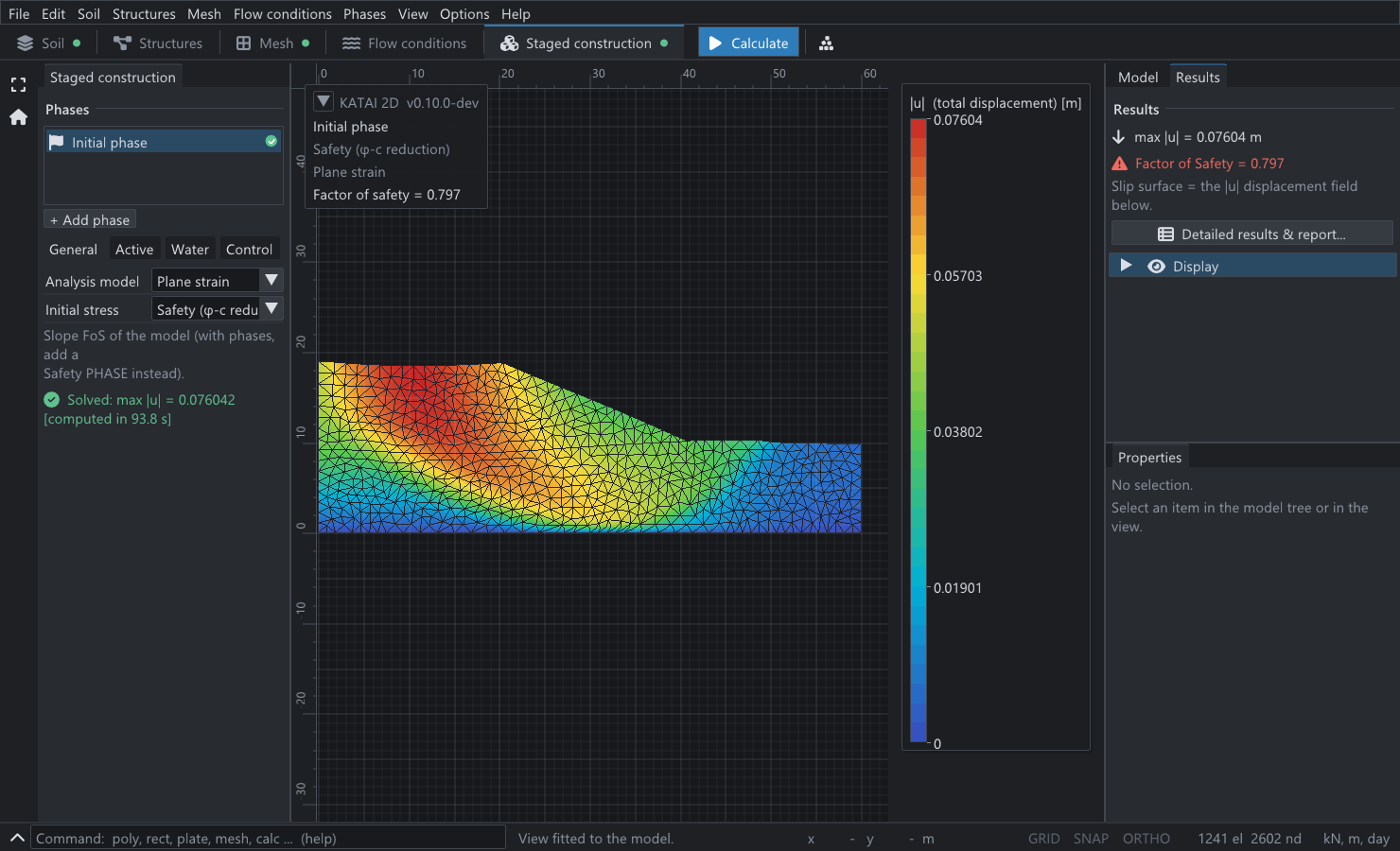
Both finite element values are below Taylor’s, and the sign is the one to expect. Taylor’s method takes a circular arc and finds the worst one. For a soil a rigid rotation about the centre of a circle is a kinematically admissible collapse mechanism, so by the upper bound theorem of plasticity each of Taylor’s values is an upper bound on the true factor of safety — the true mechanism, which is not required to be a circle, can only be as critical or more so. A finite element solution is free to find a non-circular mechanism, and Figure 1 shows that it does: the deep-seated surface flattens along the firm base rather than curving through it.
The paper states its own finite element factors only to the nearest 0.05, and describes the homogeneous case as close to Taylor’s 1.47. The values here are consistent with that reading; they are not a digit-for-digit reproduction, and the paper’s eight-node quadrilateral mesh is not the mesh used here.
3.2 Where the mechanism changesPermalink to “3.2 Where the mechanism changes”
The corner in the table can be located without drawing anything. On the base-failure branch the last full step, from a ratio of 1.00 to 1.25, raises the factor by 0.2990, a slope of 1.196 per unit of ratio. Continuing that line from 1.7276 at a ratio of 1.25 until it meets the toe-failure value of 2.0063 gives
The paper puts the transition at approximately 1.5, and notes — as these numbers also show — that the lower soil must be about half as strong again as the upper one before the toe mechanism becomes the critical one. At the ratio of exactly 1.5 the computed factor, 2.0031, is already within 0.2% of the plateau: the two mechanisms are competing, and the paper’s deformed mesh for that case shows both trying to form at once.
3.3 What a weak foundation costsPermalink to “3.3 What a weak foundation costs”
Read the table once more as an engineer rather than as a verifier. Halving the foundation strength, from a ratio of 1 to 0.5, takes the factor of safety from 1.4286 to 0.8028 — a loss of 43.8%, and a slope that was standing is not. Doubling it, from 1 to 2, gains 40.4% and then the improvement stops completely. Money spent strengthening a foundation beyond one and a half times the strength of the embankment buys nothing, and no amount of it will raise the factor above 2.0063: past that point the slope itself is the weak part.
That asymmetry is invisible if the analysis only ever looks for one kind of slip surface.
4. Why this example matters for the methodPermalink to “4. Why this example matters for the method”
A limit equilibrium search finds the minimum over the surfaces it is given. Run with base circles only, it would continue the first branch of the table upwards for ever, reporting factors of safety well above 2 for a strong foundation. Run with toe circles only, it would report about 2.1 for every ratio, including the ones where the slope has already failed through its foundation at 0.8. Either mistake is easy to make and neither produces a warning.
The finite element model was not told about either family. It was given a geometry and two strengths, and the mechanism — and the point at which it changes — came out of the equilibrium equations.
Because the soil here has and no dilatancy, the flow rule is associated and the collapse load of the discrete problem is well defined. This is the favourable case for strength reduction. With friction and a dilatancy angle smaller than the friction angle the factor becomes mesh-dependent, which KATAI 2D reports on every such run; none of the eight analyses here raised that diagnostic.
5. What this does and does not establishPermalink to “5. What this does and does not establish”
- It establishes that the strength reduction in KATAI 2D finds both mechanisms without being told about either, places the change between them at a strength ratio of 1.48 against a published value of about 1.5, and gives factors 2.8% and 4.5% below the two circular-arc upper bounds it is bracketed by.
- It does not establish the exact collapse factors. The reference values are Taylor’s chart values, which are upper bounds, read to two decimals; the paper’s own finite element values are quoted to the nearest 0.05.
- The mesh moves the numbers by about one percent. The table is for an unstructured mesh of 2576 nodes. Two of the cases were rerun on a mesh of 5660 nodes (target size 1.0 m): the homogeneous case gave 1.4248 instead of 1.4286, a change of −0.27%, and the ratio of 2 gave 1.9796 instead of 2.0063, a change of −1.33%. Both moved down, as a displacement finite element model approaching a collapse load from above must, and the toe mechanism — a thinner band of shearing — is the more sensitive of the two.
- Total stress, undrained. The example says nothing about the drained stability of the same slope, which is a different problem with different governing strengths.
6. Reproducing thisPermalink to “6. Reproducing this”
| What | Where |
|---|---|
| Script | two_layer_clay_slope.py |
| Project files, one per ratio | 0.5 · 0.75 · 1 · 1.25 · 1.5 · 1.75 · 2 · 3 |
| Program | KATAI 2D 0.9.0, the published wheel, in a clean virtual environment |
| Run time | about three minutes per ratio on a 2017 laptop |
The project files run from the command line with katai solve, and open in the desktop
application, where the two mechanisms of Figures 1 and 2 can be seen by changing one
cohesion. Every figure quoted on this page is recomputed from its stated inputs by a
script that runs on each build of this site.
ReferencesPermalink to “References”
- Griffiths, D. V. & Lane, P. A. (1999). Slope stability analysis by finite elements. Géotechnique 49(3), 387–403. — Example 4, its geometry, the strength ratio at which the mechanism changes, and the two Taylor values quoted here.
- Taylor, D. W. (1937). Stability of earth slopes. Journal of the Boston Society of Civil Engineers 24, 197–246. — the stability charts.
- Drucker, D. C. & Prager, W. (1952). Soil mechanics and plastic analysis or limit design. Quarterly of Applied Mathematics 10(2), 157–165. — the bound theorems.
- KATAI 2D 0.9.0. github.com/fkkarakurt/katai2d, Apache-2.0. doi.org/10.5281/zenodo.20692282.